Artur Sepp Blog on Quantitative Investment Strategies

  • Blog
  • Research
  • About
  • Category: Volatility Modeling

    • Lognormal Stochastic Volatility – Youtube Seminar and Slides

      Posted at 6:14 am by artursepp, on October 25, 2024

      I would like to share the youtube video of my online seminar at Minnesota Center for Financial and Actuarial Mathematics and presentation slides.

      I discuss the motivation behind introducing Karasinki-Sepp log-normal stochastic volatility (SV) model in our IJATF paper with Parviz Rakhmonov. I briefly highlight the advantages of this model over existing SV models. Then I focus on new features of the model.

      For the first time, I formulate the dynamic of log-normal SV model consistent with the forward variance by construction. This formulation enables to automatically fit the model to a given term structure of variance swap strikes implied from market prices. I show that there is a small modification of the closed-form solution presented in our paper so that the existing solution can be applied here as well.

      Also for the first time, I introduce the rough formulation of the log-normal SV model. I note that our exponential affine expansion for the classic log-normal SV model can also be applied for the rough version, but it results in a system of multi-variate system of integral equations which is numerically tedious. We need to resort tom Monte-Carlo simulations of this model and Deep Learning for model calibration. This is work in progress so stay tuned.

      Finally, I present the model calibration to the time series of implied volatilities of options on Bitcoin traded on Deribit. I touch upon the calibration of mean-reversion parameters using empirical auto-correlation function discussed in our paper. The rest of model parameters: the current level and long-term mean volatility, volatility beta, and volatility-of-volatility are fitted in time series calibration.

      Below I show that the model error (the average difference between market and model implied volatility) is less than 1% most of the times. The volatility beta serves as the expected skeweness indicator switching from large negative values during risk-aversion and positive values during risk-seeking periods. This time series construction can serve as a base for relative value analysis and quant trading strategies.

      I mention that Python implementation of model is available in stochvolmodels package at Github. See an example of running the log-normal SV model and example of model calibration using the new formulation of term structure consistent with impled variance.


      Disclosure

      This research is a personal opinion and it does not represent an official view of my current and last employers.

      This paper and the post is an investment advice in any possible form.

      Share this:

      • Share on LinkedIn (Opens in new window) LinkedIn
      • Share on X (Opens in new window) X
      • Share on WhatsApp (Opens in new window) WhatsApp
      • Email a link to a friend (Opens in new window) Email
      • Print (Opens in new window) Print
      Posted in Crypto, Python, Volatility Modeling, Volatility Trading | 2 Comments
    • Unified Approach for Hedging Impermanent Loss of Liquidity Provision – Research paper

      Posted at 7:16 pm by artursepp, on July 9, 2024

      Let me introduce our research paper co-authored with Alexander Lipton and Vladimir Lucic for hedging of impermanent loss of liquidity provision (LP) staked at Decentralised Exchanges (DEXes) which employ Uniswap V2 and V3 protocols.

      Uniswap V3 protocol allows liquidity providers to concentrate liquidity in specified ranges. As a result, the liquidity of the pool can be increased in certain ranges (typically around the current price) and the potential to generate more trading fees from the LP is increased accordingly. I illustrate the dynamics of staked LP using ETH/USDT pool as an example. A liquidity provider stakes liquidity to a specific range using initial amount of ETH and USDT tokens as specified by Uniswap V3 CFMM. When the price of ETH falls, traders use the pool to swap USDT by depositing ETH, so that the LP accrues more units of ETH. Thus when ETH falls persistently, the liquidity provider ends up holding more units of the depreciating asset, which is similar to being short a put option. In opposite, when ETH price increases, traders will deplete ETH reserves from the pool by depositing
      USDT tokens. Thus, the liquidity provider ends up holding less units of the appreciating asset, which is similar to being short a call option. The combined effect of increasing / decreasing the exposure to depreciating / appreciating asset leads to what is known as the impermanent loss in Decentralised Finance (DeFi) applications.

      In Figure 1, I show ETH units (left y-axis) and USDT units (right y-axis) for LP on Uniswap V3 with 1m USDT notional and p_{0}=2000, p_{a}=1500, p_{b}=2500. The initial LP units of (ETH, USDT) are (220, 559282). The red bar at p=1500 shows LP units of (543, 0) with LP fully in ETH units when price falls below lower threshold p_{a}. The
      green bar at $p=2500$ shows corresponding LP units of (0, 1052020) with LP fully in USDT units when price rises above upper threshold p_{b}. In subplot (B), we show USDT values of 50%/50% ETH/USDT portfolio, Funded LP positions (funded LP involves the purchase of ETH for staking without any delta hedge) and Borrowed LP positions (Borrowed LP is produced by static delta hedge of the initial staked position in ETH).

      The value profile of funded LP resembles the profile of a covered call option (long ETH and short out-of-the-money call). The value of the borrowed LP resembles the payoff of a short straddle (short both at-the-money call and put).

      Figure 1. The impremanent loss of funded and borrowed LP position

      (A) ETH units (left y-axis) and USDT units (right y-axis) for LP on Uniswap V3. (B) USDT value of 50%/50% ETH/USDT portfolio, Funded LP position and Borrowed LP position. Uniswap V3 LP position is constructed using 1m USDT notional with p_{0}=2000, p_{a}=1500, p_{b}=2500.


      We define the protection claim against the impermanent loss (IL) as a derivative security whose payoff at time T equals to negative value of the IL.

      We develop static model-independent and dynamic model-dependent approaches for hedging of the IL of liquidity provision (LP) staked at Decentralised Exchanges (DEXes) which employ Uniswap V2 and V3 protocols.

      For staking of BTC and ETH with liquid options market, the liquidity provider can apply out static model-independent replication to eliminate the IL completely.

      In Figure 2, I illustrate the replicating of IL for borrowed Uniswap V3 LP. I use strikes with widths of 50 USDT in alignment with ETH options traded on Deribit exchange (for options with maturity of less than 3 days, Deribit introduces new strikes with widths of $25$). In subplot (A), I show the IL of the borrowed LP position, and the payoffs of replicating calls and puts portfolios (with negative signs to align with the P&L). In subplot (B), we show the residual computed as the difference between the IL and the payoff of the replication portfolios. In Subplot (C), I show the number of put and call option contracts for the replication portfolios. It is clear that the approximation error is zero at
      strikes in the grid, which is illustrated in subplot (B). The maximum value of the residual is 0.025% or 2.5 basis points, which is very small. A small approximation error with a similar magnitude will occur in case, p_{0}, p_{a}, p_{b} are not placed exactly at the strike grid.

      Figure 2. Replication of IL of borrowed Uniswap V3 LP for allocation of 1m USDT notional, p_{0}=2000 ETH/USDT with p_{a}=1500 and p_{b}=2500. (A) Impermanent loss in USDT and (negative) values of replicating puts and call portfolios; (B) Residual, which is the spread between IL and options replication portfolios; (C) Number of option contracts for put and calls portfolios.


      For cryptocurrencies without a liquid options market develop the model-dependent valuation and dynamics hedging of IL protection claims for Uniswap V2 and V3 protocols. Model-based valuation can be employed by a few crypto trading companies that currently sell over-the-counter IL protection claims. When using model-based dynamics delta-hedging for the replication of the payoff of the IL protection claim, the profit-and-loss (P&L) of the dynamic delta-hedging strategy will be primarily driven by the realised variance of the price process. Thus, the total P&L of a trading desk will be the difference between premiums received (from selling IL protection claims) and the variance realised through delta-hedging. Trading desk can employ our results for the analysis of price dynamics and hedging strategies which optimize their total P&L.

      The simplest dynamic model is of course the Black-Scholes-Merton model which allows to analyze the sensitivity of the price for IL protection as a function of a single parameter for log-normal volatility

      In Figure 3, I show the annualised cost (APR) % for the cost of BSM hedge for the borrowed LP as a function of the range multiple m such that p_{a}(m)=e^{-m}p_{0} and p_{b}(m)=e^{m}p_{0}. I use two weeks to maturity T=14/365 and different values of log-normal volatility \sigma. All being the same, it is more expensive to hedge
      narrow ranges.

      Figure 3. BSM premium annualised (U^{borrower}(t, p_{t})/T) for borrowed LP with time to maturity of two weeks and notional of 1 USDT as function of the range multiple m such that p_{a}(m)=e^{-m}p_{0} and p_{b}(m)=e^{m}p_{0}.


      Further, we consider a wide class of dynamics models with jumps and stochastic volatility for which the moment generating function (MGF) for the log-return  is available in closed-form. The closed-form solution for the MGF is available under a wide class of models including jump-diffusions and diffusions with stochastic volatility. Thus, we can
      develop analytic solution for model-dependent valuation of IL protection under various models with analytic MGF.

      In particular, we apply the log-normal SV model which can handle positive correlation between returns and volatility observed in price-volatility dynamics of digital assets (see my paper with Parviz Rakhmonov for details).

      In Subplot (A) of Figure 4, I show the implied volatilities of the log-normal SV model for a range of volatility of residual volatility with zero volatility beta (which is typical for ETH skews). In Subplot (B), I show the premium APR for IL protection as a function of range multiple for a range of volatility-of-volatility. We see that the model-value of IL protection is is not very sensitive to tails of implied distribution (or, equivalently, to the convexity of the implied volatility). The reason is that the most of the value of IL protection is derived from the center of returns distribution.

      Figure 4. (A) BSM volatilities implied by log-normal SV model as function of volatility-of-volatility parameter ; (B) Premiums APR computed using log-normal SV model for borrowed LP as function of the range multiple m such that p_{a}(m)=e^{-m}p_{0} and p_{b}(m)=e^{m}p_{0}.

      For liquidity providers, who buy IL protection claims for their LP position, the total P&L will be driven by the difference between accrued fees from LP positions and costs of IL protection claims. The cost of the IL protection claim can be estimated beforehand using either the cost of static options replicating portfolio or costs of buying IL protection from a trading desk. As a result, liquidity providers can focus on selecting DEX pools and liquidity ranges where expected fees could exceed hedging costs. Thus, liquidity providers can apply our analysis optimal allocation to LP pools and for creating static replication portfolios using either traded options or assessing costs quoted by providers of IL protection.

      We leave the application of our model-free and model-dependent results for an optimal liquidity provision and optimal design of LP pools for future research.

      Enjoy reading the paper available on SSRN https://papers.ssrn.com/sol3/papers.cfm?abstract_id=4887298

      Share this:

      • Share on LinkedIn (Opens in new window) LinkedIn
      • Share on X (Opens in new window) X
      • Share on WhatsApp (Opens in new window) WhatsApp
      • Email a link to a friend (Opens in new window) Email
      • Print (Opens in new window) Print
      Posted in Crypto, Decentralized Finance, Uncategorized, Volatility Modeling | 1 Comment
    • Log-normal stochastic volatility with quadratic drift – open access publication

      Posted at 5:01 pm by artursepp, on March 7, 2024

      Our article “Log-normal Stochastic Volatility Model with Quadratic Drift” co-authored with Parviz Rakhmonov is published in International Journal of Theoretical and Applied Finance with open access https://www.worldscientific.com/doi/10.1142/S0219024924500031

      The log-normality of realised and implied volatilities of asset returns is a well-documented empirical feature. For example, see Christoffersen-Jacobs-Mimouni (2010) for equity indices and Andersen-Lund (1997) for short-term interest rates. Yet, the difficulty in implementing log-normal stochastic volatility (SV) models in practice is that these models are not analytically tractable due to being non-affine, so that standard techniques for affine SV model cannot be applied here. Our key contribution is the closed-form accurate and fast approach for valuation of vanilla options under the log-normal SV model.

      I have started working on the log-normal SV model back in 2012 together with Piotr Karasinski and we published a joint paper in Risk. Over years, I have developed the affine expansion for log-normal SV model which is analytic (up to solving a system of ODEs) and which provides a very accurate solution to the moment generating function (MGF) arising in log-normal SV models. Be means of this solution to the MGF, we can value vanilla options using methods developed for valuation under affine models, including the Lipton-Lewis formula.

      With Parviz, we have extended Karasinki-Sepp stochastic volatility model by adding a quadratic mean-reversion to the drift, which turns to be important for the model to be functionally invariant under different numeraire measures (see our paper on this topic). We have provided detailed proofs on important aspect of our model including the positivity and finiteness of the volatility process, the martingality of the price dynamics, the existence of the solution for valuation equation in this model, and the stability of the affine expansion. The most parts of our paper are technical to address these necessary topics.

      We have also included the illustration of model calibration to options data on Bitcoin from April 2019 to October 2023. For this extended period, we show that the model can fit accurately to the market data across different market regimes with low/high volatilities, positive/negative skews, and  steep/flat convexities of market implied volatilities.

      A big advantage of using the log-normal SV model in a traditional quant valuation setup, it that the model is easy to implement for Monte-Carlo (MC) simulations and for numerical PDE solvers using the the logarithm of the volatility as a modelling variable, which is defined on unrestricted domain. In contrast, affine models require to handle the positivity of the volatility in MC simulations and PDEs solvers, which is not trivial. The availability of closed-form solution for vanilla options enables fast model calibration to market data.

      Finally, our log-normal SV model is conceptually robust because if can be applied for valuation of derivatives on different asset classes. In particular, we apply this model to interest rates (see application to Cheyette model here and to Factor HJM model here), whereas traditional SV models have many limitations when it comes to modeling dynamics of fixed income  derivatives.

      For transparency and as a courtesy to the readers, Python implementation of the analytics from the paper for valuation under our log-normal SV model is available in Github.

      Enjoy reading and testing our model.

      Share this:

      • Share on LinkedIn (Opens in new window) LinkedIn
      • Share on X (Opens in new window) X
      • Share on WhatsApp (Opens in new window) WhatsApp
      • Email a link to a friend (Opens in new window) Email
      • Print (Opens in new window) Print
      Posted in Volatility Modeling | 2 Comments
    • AD Derivatives podcast on volatility modeling and DeFi

      Posted at 7:28 pm by artursepp, on December 7, 2023

      I had a pleasure talking with Greg Magadini from Amberdata Derivatives. Greg is a seasoned options trader and he co-founded of GVol which provides awesome analytics for crypto options: check it out!

      We discussed many interesting topics including my background in becoming a quant, volatility modelling and trading, and my latest work in crypto options and DeFi.

      Greg put a nice summary to get you engaged

      https://blog.amberdata.io/ad-derivatives-podcast-feat-artur-sepp-head-quant-at-clearstar-labs

      and to watch the podcast on Youtube

      https://www.youtube.com/watch?v=3Km02FDIpxM

      Enjoy!

      Share this:

      • Share on LinkedIn (Opens in new window) LinkedIn
      • Share on X (Opens in new window) X
      • Share on WhatsApp (Opens in new window) WhatsApp
      • Email a link to a friend (Opens in new window) Email
      • Print (Opens in new window) Print
      Posted in Crypto, Uncategorized, Volatility Modeling, Volatility Trading | 0 Comments
    • What is a robust stochastic volatility model – research paper

      Posted at 4:38 pm by artursepp, on November 28, 2023

      I would like to share my research and thoughts about stochastic volatility models and, in particular, about the log-normal stochastic volatility model that I have been developing in a series of papers (see introductory paper with Piotr Karasinski in 2012, the extension to include quadratic drift with Parviz Rakhmonov in 2022, and application of the model to Cheyette interest rate model and  to factor HJM framework.

      In my new working paper with Parviz Rakhmonov, which is available on SSRN here, we address specification of the functional form for the dynamics of stochastic volatility (SV) driver including affine, log-normal, and rough specifications. We propose the four principles which, in our opinion, determine the applicability of an SV model for valuation of derivative securities for different asset classes including equities, rates, commodities, FX and cryptocurrencies. We emphasise that the invariance of an SV under different numeraires is crucial for the model applications for modeling volatility of different asset classes. We argue that currently only the two SV dynamics satisfy these universality conditions: affine Heston SV model and log-normal SV model with quadratic drift. We discuss that both models are analytically tractable for valuation of vanilla options and model calibration when applying these models in different asset classes. We also present some empirical evidence for the considered models and discuss their link with contemporary research topics such as volatility skew-stickiness. We conclude that log-normal SV model with quadratic drift is robust because it does not require special conditions (such as Feller condition for Heston model) for numerical implementation of the model using MC and PDE methods.

      For illustrations, we use the implied volatilities of the core assets for equity indices, rates and commodities:

      1.  S&P 500 index and its implied volatilities proxied with VIX index;

      2. 10y US treasury rate and its implied volatilities proxied with MOVE index;

      3. Oil futures (using USO ETF) and its implied volatilities proxied with OVX index;

      4. Bitcoin (denoted as BTC) and its implied at-the-money (ATM) volatility for options with time-to-maturity of 7 days (We use historical options data of Deribit exchange with the data set starting on April 2019).

      We formulate the following principles for universality and feasibility of a stochastic volatility (SV) model. Our primary focus is based on specifying the parametric form of the dynamics of the volatility driver so that we leave aside important but, in our opinion, secondary features of a universal volatility model including jumps, local volatility, etc.

      1. The dynamics of volatility must have the same marginal distribution under statistical measure P and risk-neutral valuation measure Q. This point ensures that the model can be used under the both statistical and pricing measures. More generally, this requirement implies that the model can be used with different numeraires specific to different asset classes, including equities, rates, commodities, FX and cryptocurrencies. For universality of a SV driver, the SV model dynamics must be functionally invariant     under different numeraires. For an example, for interest rates derivatives it is necessary that the volatility dynamics are invariant under the annuity measure, while for options on FX and cryptocurrencies the model must be invariant under the price numeraire.

      2. The price process augmented with stochastic volatility must remain a strict martingale under different model specification. This particular point is important for the model application for assets with positive implied volatility skews and, as a result, with positive return-volatility correlation.

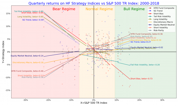
      Lions and Musiela in their 2007 paper  show that most of one-factor SV models fail to produce strict martingale dynamics when return-volatility correlation between SV and return drivers is positive. This point can be overlooked in equity derivatives where return-volatility correlation is strongly negative but it cannot neglected for other asset classes where return-volatility is positive on many occasions. In Figure 1, we show that volatility beta may become positive (so that return-volatility correlation is positive too) for interest rates and commodities. We show here that return-volatility correlation may become positive for cryptocurrencies too.

      Figure 1: Volatility beta estimated using EWMA regression model with span of 65 days: (A) time series from inceptions, (B) Empirical PDF


      3. The dynamics of volatility must be well behaved: the volatility process must be strictly positive without explosions, the stationary distribution of the volatility must exist. This point ensures that the model can implemented efficiently with analytical and numerical methods.

      4. The model is relatively easy to implement both analytically (for model calibration to market data) and numerically (through Monte-Carlo and PDEs) for valuation of exotic options and structured products.

      We make the following conclusions about our four principals applied to well-known SV models (the references are given in our paper).

      Stein-Stein SV model does not admit a valid change of measure. While it is still possible to use this model by directly specifying it under either Q or P measures, the scope of the model is limited. For example price numeraire (for FX and cryptocurrency derivatives) or annuity numeraire (for interest rate derivatives) cannot be applied for this model.

      Exp-OU SV model, Bergomi one-factor model, and log-normal volatility model with linear drift allow for change of measures, but the functional form of model dynamics changes because of an additional term which arises in the drift of the volatility due to measure change. These models do not admit strong martingale dynamics when  return-volatility correlation is positive. In our opinion, these models are originally designed for applications in equity derivatives and their application to other asset classes is rather limited.

      Rough SV model is an extension of Exp-OU using the power kernel for Brownian driver in the volatility dynamics. While rough volatility may provide good fit to empirical auto-correlation function (ACF) as we show in the Figure 2 below, the marginal improvement over a one-factor SV model is rather low when using ACF fit metric (the absolute difference is less than 0.1). Rough OU-based SV models inherit drawbacks of Exp-OU models: first, the difficulty in changing measures consistently and, second, the lack of martingale property when return-volatility correlation is positive. In our opinion, rough SV models are designed exclusively for equity markets and it may not be feasible to apply them for other asset classes. On the implementation side, rough Exp-OU models can only be implemented with MC methods.

      Figure 2: Auto-correlation of implied volatilities as function of lag periods (in days) for the three implies volatility indices: A) VIX for the S&P 500 index, B) MOVE for the 10y UST rate, C) OVX for oil ETF, D) Bitcoin (BTC) ATM implied volatilities for options with maturities of 7 day. Empirical is the empirical estimate, Log SV is the fitted auto-correlation of the lognormal SV model, Rough is the rough auto-correlation with fitted decay power alpha.


      Heston SV model allows for consistent measure changes under different numeraires. The model also produces true martingale dynamics when return-volatility correlation is positive and the variance cannot hit zero as long as the Feller condition is satisfied. On the implementation side, Heston model admits a closed-form solution for valuation of vanilla options, which makes it easy for model calibration. These facts undoubtedly have made Heston model applicable to multiple asset classes. However, numerical implementation of Heston model using MC or numerical PDE methods is rather complicated, especially when Feller condition is not satisfied. There is a great deal of literature on how to make Heston model work in practice.

      Heston model also implied the stationary distribution of the volatility which has a thin right tail which is inconsistent with empirical data shown in Figure 3 below.

      Figure 3: Steady-state PDF of the logarithm of the volatility (y-axis is shown in log-scale).


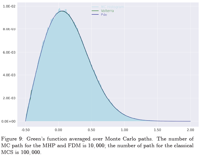
      Log-normal SV model with quadratic drift allows for consistent measure changes using different numeraires. For positive return-volatility correlation, the model produces true martingale dynamics as long as the quadratic mean-reversion coefficient exceeds volatility beta. For model calibration, we develop a closed-form and accurate solution for valuation of vanilla options under this model in this paper. For numerical implementation using MC methods, we also develop a first-order MC scheme using the log-transform of the volatility to unbounded domain. Since in log-coordinates the valuation problem in log-volatility is defined on unrestricted domain, the problem can be solved efficiently using PDE methods for such domain (see my old workshop slides here). As a result, log-normal SV model with quadratic drift can be considered as a robust choice for modeling price dynamics for different asset classes.

      Enjoy the reading of our paper in full and feel free to provide comments.

      Python code for producing figures is available on Github in stochvolmodels package https://github.com/ArturSepp/StochVolModels and in module for the paper https://github.com/ArturSepp/StochVolModels/tree/main/my_papers/volatility_models

      Share this:

      • Share on LinkedIn (Opens in new window) LinkedIn
      • Share on X (Opens in new window) X
      • Share on WhatsApp (Opens in new window) WhatsApp
      • Email a link to a friend (Opens in new window) Email
      • Print (Opens in new window) Print
      Posted in Volatility Modeling | 2 Comments
    • Robust Log-normal Stochastic Volatility for Interest Rate Dynamics – research paper

      Posted at 5:49 pm by artursepp, on December 31, 2022

      The volatility of interest rates in 2022 has been indeed extreme. In Figure 1, I show the dependence the between the MOVE index (which measures the implied volatility of one-month options on UST bond futures and which is constructed similarly to the VIX index for implied volatilities of the S&P index futures), realized 10y UST rate volatility over the 6 months rolling window, and the level of 10y UST rates. For understanding of historical patterns, we classify the historical period from 2002 to the end of 2022 into the 5 periods: 2002-2007 (hiking cycle), 2008-2010 (tightening), 2011-2017 (QE), 2018-2020 (tightening), 2021-2022 (hiking cycle).

      We see that period of 2021-2022 was indeed unprecedented period when the rates rose from low levels of around 100 basis point (bp) to over 400bp, while the rates implied and realised volatilities rose from 50bps to over 150bps.

      Figure1. (A) The MOVE implied volatility index vs 10y UST bond rate; (B) 6m realized volatility of 10y UST bond rate vs 10y UST bond rate.

      The dependence between the rate and its volatility manifests in implied volatilities with positive skews as I show in Figure 2 (The market convention is to use Bachelier normal model for marking implied swaption volatilities).

      Figure 2. Implied normal volatilities for $10Y$ swaption as function of option expiries in basis points observed in December 2022. Option delta is Bachelier normal model delta.

      The dependence between the rate and volatility also manifests in strong level between the implied and realized volatilities and the volatility of volatility and the volatility beta (the change in 1bp of the volatility predicted by 1bp change in rates) which I show in Figure 3.

      Figure 3. (A) Realized volatility-of-volatility vs move volatility index. (B) Realized volatility beta vs Move index.

      Quantitative modeling of such dynamics is challenging. In my previous joint paper with Parviz Rakhmonov on the
      log-normal stochastic volatility for assets with positive return-volatility correlation we show that conventional SV model are ill-equipped for such dynamics. The rate dynamics are no exception, and practitioners rely on either local volatility models or local SV models with zero correlation. Both approaches are ill-poised because the may lead to explosive behavior of interest rates.

      In our extension with Parviz we apply the Karasinski-Sepp log-normal SV dynamic for modelling the interest rate volatility, which is available on SSRN: Robust Log-normal Stochastic Volatility for Interest Rate Dynamics

      We show that the proposed rates model is robust both on the quantitative dynamics and its practical implementation. While rate models in general are notorious for their tractability and implementation, we derive a closed form analytic solution for valuation of swaptions and for model calibration. In Figure 4, I show the model implied distribution of the 10y swap rate in the annuity measure computed using our analytical methods compared to the Monte Carlo simulations. Our solution is very accurate and it allows for robust calibration of the model to market data.

      Figure 4. Probability density functions computed using the first order affine expansion and the second-order expansion for the distribution of 10y swap rate in one year. The blue histogram is computed using realizations from MC simulations in model dynamics.

      All the technical details are available in the paper: Robust Log-normal Stochastic Volatility for Interest Rate Dynamics. Happy reading.

      Share this:

      • Share on LinkedIn (Opens in new window) LinkedIn
      • Share on X (Opens in new window) X
      • Share on WhatsApp (Opens in new window) WhatsApp
      • Email a link to a friend (Opens in new window) Email
      • Print (Opens in new window) Print
      Posted in Quantitative Strategies, Volatility Modeling, Volatility Trading | 1 Comment
    • Log-normal Stochastic Volatility Model for Assets with Positive Return-Volatility Correlation – research paper

      Posted at 3:04 pm by artursepp, on August 10, 2022

      I am introducing my most recent research on log-normal stochastic volatility model with applications to assets with positive implied volatility skews, such as VIX index, short index ETFs, cryptocurrencies, and some commodities.

      Together with Parviz Rakhmonov, we have extended my early work on Karasinski-Sepp log-normal volatility model and we have written an extensive paper with an extra focus on modelling implied volatilities of assets with positive return-volatility correlation in addition to deriving a closed-form solution for option valuation under this model.

      Assets with positive implied volatility skews and return-volatility correlations

      While it is typical to observe negative correlation between returns of an asset and changes in its implied and realized volatilities, there are in fact many assets with positive return-volatility correlation and, as a consequence, with positive implied volatility skews. In below Figure, I show some representative examples.

      (A) The VIX index provides protection against corrections in the S&P 500 index, so that out-of-the-money calls on VIX futures are valuable and demand extra risk-premia than puts.

      (B) Short and leveraged short ETFs on equity indices have positive implied volatility skews because of their anti-correlation with underlying equity indices. I use 3x Short Nasdaq ETF with NYSE ticker SQQQ, which is the largest short ETF in US equity market and which has very liquid listed options market.

      (C) Cryptocurrencies, including Bitcoin and Ethereum, and “meme” stocks, such as AMC, have positive skews during speculative phases when positive returns feed speculative demand for upside. These self-feeding price dynamics increase the demand for calls following a period of rising prices. However, positive return-volatility correlation tend to reverse once “greed” regime is over and “risk-off” regime prevails.

      (D) Gold and commodities in general may have positive volatility skews dependent on supply-demand imbalances, seasonality, etc.

      Importantly, the valuation of options on these assets is not feasible using conventional stochastic volatility models applied in practice such as Heston, SABR, Exponential Ornstein-Uhlenbeck stochastic volatility models, because these models fail to be arbitrage-free (forwards and call prices are not martingals). Curiously enough, the topic of no-arbitrage for SV models with positive return-volatility correlation has not received attention in literature, despite a large number of assets with positive return-volatility correlation.

      Applications to Options on Cryptocurrencies

      Additional, yet important application of our work is the pricing of options on cryptocurrencies, where call and put options with inverse pay-offs are dominant. The advantage of inverse pay-offs for cryptocurrency markets is that all option-related transactions can be handled using units of underlying cryptocurrencies, such as Bitcoin or Ethereum, without using fiat currencies. Critically, since both inverse options (traded on Deribit exchange) and vanilla (traded on CBOE) are traded for cryptocurrencies, a stochastic volatility must satisfy the martingale condition for both money-market-account and inverse measures to exclude arbitrage opportunities between vanilla and inverse options. We show that prices dynamics in our model are martingales under the both inverse and money-market-account measures.

      In below Figure, I show the model fit to Bitcoin options observed on 21-Oct-2021 (the period with positive skew) for most liquid maturities of 2 weeks, 1 month, and 2 and 3 months. We see that the model calibrated to Bitcoin options data is able to capture the market implied skew very well across most liquid maturities with only 5 model parameters. The average mean squared error (MSE) is about 1% in implied volatilities, which is mostly within the quoted bid-ask spread. Calibration to ATM region can be further improved using a term structure of the mean volatility or augmenting the SV model with a local volatility part to fit accurately to the implied volatility surface.

      Model applications

      The quality of model fit is similar for other assets with either positive or negative skews. The main strength of our model is that it can be used for the following purposes.

      1. Cross-sectional no-arbitrage model for different exchanges and options referencing the same underlying.
      2. Model for time series analysis of implied volatility surfaces.
      3. Dynamic valuation model for structured products and option books.

      Further resources

      SSRN paper Log-normal Stochastic Volatility Model with Quadratic Drift https://ssrn.com/abstract=2522425

      Github project with the example of model implementation in Python: https://github.com/ArturSepp/StochVolModels

      Youtube video with lecture I made at Imperial College for model applications for Bitcoin volatility surfaces: https://youtu.be/dv1w_H7NWfQ

      Youtube podcast with introduction of the paper and review of Github project with Python analytics for model implementation: https://youtu.be/YHgw0zyzT14

      Disclaimer

      The views and opinions presented in this article and post are mine alone. This research is not an investment advice.

      Share this:

      • Share on LinkedIn (Opens in new window) LinkedIn
      • Share on X (Opens in new window) X
      • Share on WhatsApp (Opens in new window) WhatsApp
      • Email a link to a friend (Opens in new window) Email
      • Print (Opens in new window) Print

      Like this:

      Like Loading...
      Posted in Crypto, Python, Volatility Modeling, Volatility Trading | 1 Comment
    • Toward an efficient hybrid method for pricing barrier options on assets with stochastic volatility – research paper

      Posted at 2:00 pm by artursepp, on February 23, 2022

      I am excited to share the latest paper with Prof. Alexander Lipton.

      https://papers.ssrn.com/sol3/papers.cfm?abstract_id=4035813

      We find the semi-analytical solution to one of the unsolved problems in Quantitative Finance, which is to compute survival probabilities and barrier option values for two-dimensional correlated dynamics of stock returns and stochastic volatility of returns.

      An analytical solution to such a problem does not appear feasible because the valuation equation is asymmetric in the log-price variable when the correlation between returns and the volatility of returns is non-zero. In the case of zero correlation, an analytic closed-form solution is achievable involving a numerical integration in the Fourier space.

      In this article, we combine one-dimensional Monte Carlo simulations and the semi-analytical one-dimensional heat potential method (MHP) to design an efficient technique for pricing barrier options on assets with correlated stochastic volatility. Our approach to barrier options valuation utilizes two loops. First, we run the outer loop by generating volatility paths via the Monte Carlo method. Second, we condition the price dynamics on a given volatility path and apply the method of heat potentials to solve the conditional problem in closed-form in the inner loop. Next, we illustrate the accuracy and efficacy of our semi-analytical approach by comparing it with the two-dimensional Monte Carlo simulation and a hybrid method, which combines the finite-difference technique for the inner loop and the Monte Carlo simulation for the outer loop. Finally, we apply our method to compute state probabilities (Green function), survival probabilities, and the value of call options with barriers.

      As a byproduct of our analysis, we generalize Willard’s (1997) conditioning formula for valuation of path-independent options to path-dependent options. Additionally, we derive a novel expression for the joint probability density for the value of drifted Brownian motion and its running minimum or maximum in the case of time-dependent drift.

      Our approach provides better accuracy and is orders of magnitude faster than the existing methods. The methodology is general and can equally efficiently manage all known stochastic volatility models. Besides, relatively simple extensions (will be described elsewhere) can also handle rough volatility models. With minimal changes, one can use the method to price popular double-no-touch options and other similar instruments.

      Share this:

      • Share on LinkedIn (Opens in new window) LinkedIn
      • Share on X (Opens in new window) X
      • Share on WhatsApp (Opens in new window) WhatsApp
      • Email a link to a friend (Opens in new window) Email
      • Print (Opens in new window) Print
      Posted in Quantitative Strategies, Volatility Modeling | 0 Comments
    • Tail risk of systematic investment strategies and risk-premia alpha

      Posted at 2:55 pm by artursepp, on April 9, 2019

      Everyone knows that the risk profile of systematic strategies can change considerably when equity markets turn down and volatilities spike. For an example, a smooth profile of a short volatility delta-hedged strategy in normal regimes becomes highly volatile and correlated to equity markets in stressed regimes.

      Is there a way to systematically measure the tail risk of investment products including hedge funds and alternative risk premia strategies? Further, how do we measure the risk-premia compensation after attribution for tail risks? Finally, would we discover patterns in cross-sectional analysis of different hedge fund strategies?

      I have been working through years on a quantitative framework to analyse the above raised questions and recently I wrote two articles on the topic:

      1. The regime-conditional regression model is introduced in The Hedge Fund Journal (online paper).
      2. A short review of the methodology and results is presented for QuantMinds

      I would like to highlight the key results of the methodology so that interested readers can further follow-up with the original sources.

      Regime conditional index betas

      In the top Figure, I show the regime conditional betas for a selection of hedge fund style from HFR indices data using the S&P 500 index as the equity benchmark.

      We can classify the strategies into defensive and risk-seeking based on their return profile in bear market regimes:

      1. Defensive strategies (long volatility, short bias, trend-following CTAs) have negative equity betas in bear regime so that these strategies serve as diversifiers of the equity downside risk.
      2. Risk-seeking strategies (short volatility, risk-parity) have positive and significant equity betas in bear regime. Equity betas of most of risk-seeking strategies are relatively small in normal and bull periods but equity betas increase significantly in bear regimes. I term these strategies as Risk-seeking risk-premia strategies.
      3. I term strategies with insignificant betas in normal bear regimes as Diversifying strategies. Examples include equity market neutral and discretionary macro strategies because, even though these strategies have positive betas to the downside, the beta profile does not change significantly between normal and bear regimes. As a result, the marginal increase in beta exposure between normal and bear periods is insignificant.

      Risk-premia alpha vs marginal bear beta

      I define the risk-premia alpha as the intercept of the regime-conditional regression model for strategy returns regressed by returns on the benchmark index. To show a strong relationship between the risk-premia alpha and marginal bear beta (the marginal bear betas are computed as the difference between betas in normal and bear regimes), I apply the cross-sectional analysis of risk premia for the following sample of hedge fund indices and alternative risk premia (ARP) products, using quarterly returns from 2000 to 2018 against the S&P 500 total return index:

      1. HF: Hedge fund indices from major index providers including HFR, SG, BarclayHedge, Eurekahedge with the total of 73 composite hedge fund indices excluding CTA indices;
      2. CTA: 7 CTA indices from the above providers and 15 CTA funds specialized on the trend-following;
      3. Vol: 28 CBOE benchmark indices for option and volatility based strategies;
      4. ARP: ARP indices using HFR Bank Systematic Risk-premia Indices with a total of 38 indices.

      In figure below, I plot risk-premia alphas against marginal bear betas grouped by strategy styles. For defensive strategies, their marginal bear betas are negative; for risk-seeking strategies, the marginal bear betas are positive and statistically significant.

      cross_sectional_rp 20190405-085150

      We see the following interesting conclusions.

      1. For volatility strategies, the cross-sectional regression has the strongest explanatory power of 90%. Because a rational investor should require a higher compensation to take the equity tail risk, we observe such a clear linear relationship between the marginal tail risk and the risk-premia alpha. Defensive volatility strategies that buy downside protection have negative marginal betas at the expense of negative risk-premia alpha.
      2. For alternative risk premia products, the dispersion is higher (most of these indices originate from 2007), yet we still observe the pattern between the defensive short and risk-seeking risk-premia strategies with negative and positive risk-premia alpha, respectively.
      3. For hedge fund indices, the dispersion of their marginal bear beta is smaller. As a result, most hedge funds serve as diversifiers of the equity risk in normal and bear periods; typical hedge fund strategies are not designed to diversify the equity tail risk.
      4. All CTA funds and indices have negative bear betas with insignificant risk-premia alpha. Even though their risk-premia alpha is negative and somewhat proportional to marginal bear beta is proportional, the risk-premia alpha is not statistically significant. In this sense, CTAs represent defensive active strategies. The contributors to slightly negative risk-premia alpha may include transaction costs and management fees.


      References

      Sepp A., Dezeraud L., (2019), “Trend-Following CTAs vs Alternative Risk-Premia: Crisis beta vs risk-premia alpha”, The Hedge Fund Journal, Issue 138, page 20-31, https://thehedgefundjournal.com/trend-following-ctas-vs-alternative-risk-premia/

      Sepp, A. The convexity profile of systematic strategies and diversification benefits of trend-following strategies, QuantMinds, April 2019

      Share this:

      • Share on LinkedIn (Opens in new window) LinkedIn
      • Share on X (Opens in new window) X
      • Share on WhatsApp (Opens in new window) WhatsApp
      • Email a link to a friend (Opens in new window) Email
      • Print (Opens in new window) Print
      Posted in Asset Allocation, Quantitative Strategies, Trend-following, Uncategorized, Volatility Modeling | 1 Comment
    • My talk on Machine Learning in Finance: why Alternative Risk Premia (ARP) products failed

      Posted at 2:56 pm by artursepp, on November 27, 2018

      I have recently attended and presented at Swissquote Conference on Machine Learning in Finance. With over 250 participants, the event was a great success to hear from the industry leaders and to see the recent developments in the field.

      The conference featured very interesting talks ranging from an application of natural language processing (NLP) for industry classifications to a systematic trading in structured products using deep learning. For the interested, the slides and videos are available on the conference page.

      I would like to share and introduce my talk presented at the conference on applications of machine learning for quantitative strategies (the video of my talk available here).

      In my talk, I address the limitations of applying machine learning (ML) methods for quantitative trading given limited sample sizes of financial data. I illustrate the concept of probably approximately correct (PAC) learning that serves as a foundation to the complexity analysis of machine learning.

      In particular, the PAC learning establishes model-free bounds on the sample size to estimate a parametric function from the sample data for a specified level of approximation and estimation error. I recommend very nice textbooks An Elementary Introduction to Statistical Learning Theory and The Nature Of Statistical Learning Theory to study more about the PAC learning.

      I also present an example of using supervised learning for the selection of volatility models for systematic trading from my earlier presentation.

      Finally, I touch on the important topic of the risk-profile of quantitative investment strategies and, in particular, Alternative Risk Premia (ARP) products. For the past few years, since about 2015, the sell-side have been marketing a plethora of ARP products as “cheap” substitutes for hedge fund strategies. However, ARP products fared miserably throughout year 2018 despite the fact that most of these products were marketed as market-neutral. I wanted to share my view why ARP products failed…

      The typical creation process of ARP products is as follows. First, a research team runs multiple back-tests of “academic” risk factors (value, carry, momentum, etc) across many markets until a specific parametrization of their strategy produces a satisfactory Sharpe ratio (around 1.0 or so). Once the necessary performance target is achieved in the back-test, the research team along with a marketing team would write a research paper with economic justification of the strategy. Then the marketing team would pitch the strategy to institutional clients. If the marketing team is successful, they would raise money for the strategy. Finally, the successful strategy (out of dozens of attempted) would reach to the execution team who would implement the strategy in a trading system and execute on behalf of clients.

      The creation of ARP products serve as a prime example why we need to understand the limitations of statistical learning given limited sample sizes of financial data. Also, there is the incentive to fit a rich model to the limited sample to optimize the in-sample performance. For an example, using PAC learning, to estimate a model with 10 parameters at an approximation error within 10% we need to apply 2,500 daily observations!

      It is no coincidence that ARP product suffered a major blow once market conditions changed. As we speak, post October 2018, quants are facing a crisis of confidence.

      In the hindsight, year 2018 brought to the failure the two very popular strategies:

      1) The short volatility ETNs: the figure at the top of the post illustrates how would a naive 5-parameter regression fit the in-sample data of past two years with the accuracy of 98%, but the fitted model fails miserably in February 2018 (I posted a detailed statistical analysis of the crash).

      2) The alternative risk-premia products: the figure below shows the risk-profile of Bank Systematic Risk Premia Multi-Asset Index compiled by the Hedge Fund Research.

      In the figure below, as the predictor, I use the quarterly returns on the S&P 500 index which I condition into the three regimes: bear (16% of the sample), normal (68%), and bull (16%). Then I consider the quarterly returns on the HFR index conditional on these regimes and illustrate the corresponding regression of returns on the HFR index predicted by returns on the S&P 500 index.

      It is clear that the HFR index sells 3 puts to buy 5 calls to obtain the leveraged exposure to the S&P 500 index. Well, over the past decade these models learned to leverage the upside at the cost of selling the downside.

      BankRiskPremia.png

      The key message from my talk is that, we may be able to avoid the traps of applying machine and statistical learning methods for systematic trading strategies by understanding the theoretical grounds of the ML methods and the potential limitations of using only limited sample sizes for the estimation of these models.


      Disclaimer

      All statements in this presentation are the author personal views. The information and opinions contained herein have been compiled or arrived at in good faith based upon information obtained from sources believed to be reliable. However, such information has not been independently verified and no guarantee, representation or warranty, express or implied, is made as to its accuracy, completeness or correctness. Investments in Alternative Investment Strategies are suitable only for sophisticated investors who fully understand and are willing to assume the risks involved. Alternative Investments by their nature involve a substantial degree of risk and performance may be volatile.


      Share this:

      • Share on LinkedIn (Opens in new window) LinkedIn
      • Share on X (Opens in new window) X
      • Share on WhatsApp (Opens in new window) WhatsApp
      • Email a link to a friend (Opens in new window) Email
      • Print (Opens in new window) Print
      Posted in Quantitative Strategies, Uncategorized, Volatility Modeling, Volatility Trading | 2 Comments
    ← Older posts
    • Receive notifications of new posts by email

      Join 339 other subscribers
    • Recent Posts

      • The Science and Practice of Trend-following Systems: paper and presentation
      • Lognormal Stochastic Volatility – Youtube Seminar and Slides
      • Optimal allocation to cryptocurrencies in diversified portfolios – update on research paper
      • Unified Approach for Hedging Impermanent Loss of Liquidity Provision – Research paper
      • Log-normal stochastic volatility with quadratic drift – open access publication
      • Stochastic Volatility for Factor Heath-Jarrow-Morton Framework – research paper
      • AD Derivatives podcast on volatility modeling and DeFi
      • What is a robust stochastic volatility model – research paper
      • Robust Log-normal Stochastic Volatility for Interest Rate Dynamics – research paper
      • Optimal Allocation to Cryptocurrencies in Diversified Portfolios – research paper
      • Log-normal Stochastic Volatility Model for Assets with Positive Return-Volatility Correlation – research paper
      • Developing systematic smart beta strategies for crypto assets – QuantMinds Presentation
      • Toward an efficient hybrid method for pricing barrier options on assets with stochastic volatility – research paper
      • Paper on Automated Market Making for DeFi: arbitrage-fee exchange between on-chain and traditional markets
      • Tail risk of systematic investment strategies and risk-premia alpha
      • Trend-Following CTAs vs Alternative Risk-Premia (ARP) products: crisis beta vs risk-premia alpha
      • My talk on Machine Learning in Finance: why Alternative Risk Premia (ARP) products failed
      • Why Python for quantitative trading?
      • Machine Learning for Volatility Trading
      • Trend-following strategies for tail-risk hedging and alpha generation
    • Categories

      • Asset Allocation (10)
      • Crypto (8)
      • Decentralized Finance (5)
      • Python (4)
      • Quantitative Strategies (17)
      • Trend-following (4)
      • Uncategorized (20)
      • Volatility Modeling (18)
      • Volatility Trading (13)


Loading Comments...
 

    %d