I would like to introduce the updated draft of my paper co-authored with Vladimir Lucic and entitled “The Science and Practice of Trend-following Systems”.
Trend-following systems have been employed by many quantitative and discretionary funds, also known as commodity trading advisors (CTAs), or managed futures, since the early 1980s. Richard Dennis, a commodity trader on the CME, organised and instructed two classes of novice traders in late 1983 and 1984 with the idea that trading skills can be taught. The underlying ideas and methods included strict adherence to rule-based trading and risk-management. A few graduates of these classes created their own quantitatively-driven CTA funds and gave the rise of managed futures industry.
Lintner in 1983 provided the first evidence that managed futures deliver better risk-adjusted returns and offer strong diversification benefits for long-only portfolios. The following passage is from Lintner 1983, The Potential Role of Managed Commodity-Financial Futures Accounts (and/or Funds) in Portfolios of Stocks and Bonds:
“The combined portfolios of stocks (or stocks and bonds) after including judicious investments in appropriately selected sub-portfolios of investments in managed futures accounts (or funds) show substantially less risk at every possible level of expected return than portfolios of stock (or stocks and bonds) alone. This is the essence of the ‘potential role’ of managed futures accounts (or funds) as a supplement to stock and bond portfolios suggested in the title of this paper.”
Subsequent studies reinforce the role of managed futures for the diversification of broad long-only portfolios, so that currently many private and institutional portfolios have some exposure to managed futures.
The purpose of this paper is to provide both theoretical and practical insights about trend-following (TF) systems. Let me note that practitioners refer to implemented systematic futures-based strategies as systems or programs.
Theoretical insights
For theoretical insights, we establish regimes in which TF systems perform well. For any systematic strategy, it is important to understand under which market dynamics it is expected to out-perform or under-perform. We derive an exact analytical formula linking the performance of the TF system to the autocorrelation of instrument returns under generic processes. We show that the TF system is expected to be profitable when the autocorrelation of returns is positive even if the drift is zero. We also show that the TF system is expected to be profitable for a white noise process with a large positive or negative drift if the filter span is large.
For the illustration of obtained analytical results, we focus on fractional ARFIMA process which incorporates both short- and long-term mean reversion and / or trend features, which allows for extensive profitability analysis of TF systems.
In Figure 1, we illustrate that the TF system can be profitable if the fractional order is positive, so the dynamics are trending in the long-term. In this case, the TF system can be profitable even if the short-term dynamics are mean-reverting.
Figure 1. Panel (A) shows analytical value of expected annual return of TF system and MC confidence intervals using ARFIMA process with positive long-term memory with fractional order $d=0.02$, which implies long-term mean-reversion, with AR-1 feature phi={-0.05, 0.0, 0.05, and with zero drift. Panel (B) shows expected value of volatility-adjusted turnover and corresponding MC 95% confidence interval.

In Figure 2, we illustrate that if the fractional order is negative and dynamics are mean-reverting in the long-term, the TF system can still be profitable if drift is present and span of the filter is large.
Figure 2. Panel (A) shows analytical value of expected annual return of TF system and MC confidence intervals for ARFIMA process with negative long-term memory with fractional order d=-0.01. with AR-1 feature phi={-0.05, 0.0, 0.05} and with drift mu=0.5 (interpreted as Sharpe ratio) . Panel (B) shows expected value of volatility-adjusted turnover and corresponding MC 95% confidence interval.

Practical Insights
We have considered three distinct approaches for the construction of trend-following (TF) approaches which we term as European, American, and Time Series Momentum (TSMOM) systems. In Figure 3, we show the simulated performance of three TF systems assuming 2%/20% management/performance fees.
Figure 3. Simulated performance of of European, American and TSMOM systems along with the historical performance of SG Trend Index. Panels (A1), (B1), and (C1) show the cumulative log-performance, running drawdown, and EWMA correlations with one year span. Panel (A2i) shows risk-adjusted performance table with P.a. returns being annualised return or CAGR, Vol being annualised volatility of daily log returns, Sharpe (rf=0) being Sharpe ratio, Max DD being the maximum drawdown; Skew being the skewness of quarterly log-returns, beta and R^{2} being the the slope and R^{2} of the linear regression of monthly returns relative to 60/40 equity/bond portfolio. Panel (A2ii) shows annual returns. Panels (B2) and (B3) show one year rolling volatility-adjusted turnover and cost, respectively. The background colour is obtained by ordering the quarterly returns of the benchmark 60/40 portfolio from lowest to highest and the splitting the 16% of worst returns into the “bear” regime (pink colour), 16% of best returns into the bull regime (dark green colour), and remaining regimes into “normal” regimes (light green colour). The period of performance measurement is from 31 December 1999 to 1 June 2025.

This illustration emphasises the robustness of TF systems, as different quantitative models can provide first-order exposure to trending features of financial markets. Most CTA managers pursue to deliver outperformance over the benchmark index by second-order proprietary features including exposures to style factors (carry, value, cross-sectional momentum, etc.), risk-management (portfolio volatility targeting, asset class exposure management, etc.), operational capabilities (exposure to smaller or alternative futures markets, enhanced execution, etc.), and other risk premia (e.g. volatility carry) — see Carver 2023, Advanced Futures Trading Strategies, for a detailed overview of additional features and strategies commonly combined with managed futures.
Smart Diversification of Long-only Portfolios
We also analyse the diversification benefits of how blending of TF systems long-only portfolios with long-only portfolios. In Figure 4, we generate blended portfolios with (1-x)% weight to 60/40 Equity/Bond portfolio and with x% weight to each of the three TF systems with x varying from 0% to $100%. Blended portfolios are rebalanced quarterly and, for TF systems, we use their net performance. The initial portfolio on the left is 100%/0% blend of 60/40 portfolio and 0% TF system. The final portfolio on the right is 0%/100% blend. Hereby, we measure portfolio risk by the Bear-Sharpe ratio (the performance in 16% worst quarters of 60/40 equity / bond portfolio) and portfolio performance by total Sharpe ratio.
Figure 4. Bear-Sharpe ratio vs total Sharpe ratio for blended portfolios with (1-x)% weight to 60/40 portfolio and x% weight to each of the three TF systems. The initial portfolio on the left is 100%/0%$ blend of 60/40 portfolio and 0% TF system. The final portfolio on the right is 0%/100% blend. The specification of TF systems is the same as for generation of Figure 3.

We observe that the best combination of European and American TF systems that generates the highest Sharpe ratio is the 40%/60% combination of the 60/40 portfolio / TF system. In this case, the realised Bear-Sharpe ratio is close to zero, while the total Sharpe ratio is about 0.9, which is almost double the Sharpe ratios of its components. As we see in Figure 3, the TSMOM system has a Bear-Sharpe ratio attribution of 50% smaller than that of European and American TFs. Thus, the Bear-Sharpe ratio emphasises the diversification efficiency for long-only portfolios.
We note that, because implementation of a TF system requires only a limited capital for margin requirements of trading futures, a TF system can implemented as an overlay to 100% exposure to a long-only portfolio. If we take the 50%/50% blend (which is not far from the optimal blend 40%/60% in Figure 4 and leverage it twice, we obtain the portfolio with 100% exposure to the 60/40 portfolio and 100% exposure to a TF system. We note that recent advances in portfolio products termed “stacking alphas” or “portable alphas” (see Gordillo-Hoffstein, 2024, Return Stacking: Strategies For Overcoming A Low Return Environment) are based on the same concept of blending a fixed 100% exposure to a long-only portfolio and 100% (or similar) exposure to a TF system or a general managed futures program.
Further Applications
Our results, allow for prediction of the performance of TF systems conditional on certain dynamics, such as ARFIMA process. This could be applied for instrument selection and signal/weights adjustments.
Given that we also derive a very good approximate formulas for the expected turnover of European TF system, our results can be applied for quick optimisations of TF systems.
Finally, our “Smart Diversification” based on regime-conditional Sharpe ratios enables for design of overlays using TF systems for long-only portfolios. In particular, we show that the optimal weight, according to our “Smart Diversification”, of TF system for 60/40 portfolio is 50%. Return stacked portfolios are obtained by 2x leverage of 50%/50% blend of 60/40 portfolio / TF system.
Links
Our paper is available on SSRN: https://papers.ssrn.com/sol3/papers.cfm?abstract_id=3167787
I presented our paper at CQF Volatility and Risk conference with slides available here and Youtube video of my presentation is available here
Disclosure
This research is a personal opinion and it does not represent an official view of my current and last employers.
This paper and the post is an investment advice in any possible form.