Crypto | Artur Sepp Blog on Quantitative Investment Strategies

Category: Crypto
- Lognormal Stochastic Volatility – Youtube Seminar and Slides
  
  Posted at 6:14 am by artursepp, on October 25, 2024
  I would like to share the youtube video of my online seminar at Minnesota Center for Financial and Actuarial Mathematics and presentation slides.
  
  I discuss the motivation behind introducing Karasinki-Sepp log-normal stochastic volatility (SV) model in our IJATF paper with Parviz Rakhmonov. I briefly highlight the advantages of this model over existing SV models. Then I focus on new features of the model.
  
  For the first time, I formulate the dynamic of log-normal SV model consistent with the forward variance by construction. This formulation enables to automatically fit the model to a given term structure of variance swap strikes implied from market prices. I show that there is a small modification of the closed-form solution presented in our paper so that the existing solution can be applied here as well.
  
  Also for the first time, I introduce the rough formulation of the log-normal SV model. I note that our exponential affine expansion for the classic log-normal SV model can also be applied for the rough version, but it results in a system of multi-variate system of integral equations which is numerically tedious. We need to resort tom Monte-Carlo simulations of this model and Deep Learning for model calibration. This is work in progress so stay tuned.
  
  Finally, I present the model calibration to the time series of implied volatilities of options on Bitcoin traded on Deribit. I touch upon the calibration of mean-reversion parameters using empirical auto-correlation function discussed in our paper. The rest of model parameters: the current level and long-term mean volatility, volatility beta, and volatility-of-volatility are fitted in time series calibration.
  
  Below I show that the model error (the average difference between market and model implied volatility) is less than 1% most of the times. The volatility beta serves as the expected skeweness indicator switching from large negative values during risk-aversion and positive values during risk-seeking periods. This time series construction can serve as a base for relative value analysis and quant trading strategies.
  
  I mention that Python implementation of model is available in stochvolmodels package at Github. See an example of running the log-normal SV model and example of model calibration using the new formulation of term structure consistent with impled variance.
  
  Disclosure
  
  This research is a personal opinion and it does not represent an official view of my current and last employers.
  
  This paper and the post is an investment advice in any possible form.
  Share this:
  LinkedIn
  X
  WhatsApp
  Email
  Print
  Posted in Crypto, Python, Volatility Modeling, Volatility Trading | 2 Comments
- Optimal allocation to cryptocurrencies in diversified portfolios – update on research paper
  
  Posted at 3:08 pm by artursepp, on August 18, 2024
  Cryptocurrencies have been acknowledged as an emerging asset class with a relatively low correlation to traditional asset classes and independent drivers of their long-term performance (see for an example excellent papers by Harvey et al (2022) and Adams at al (2024)).
  
  A year ago in Summer of 2023, I published research article in Risk Magazine (SSRN draft) on quantitative methods for optimal allocation to cryptocurrencies within alternative and balanced portfolios. The metrics for consideration include metrics for portfolio diversification, expected risk-return relationships and skewness of the returns distribution. Using roll-forward historical simulations, I showed that all four allocation methods produce a persistent positive allocation to Bitcoin and Ether in alternative and balanced portfolios with a median allocation of about 2.7%.
  
  This time, I would like to present the updated outcomes from my model given that Bitcoin and Ether had a strong performance of 95% and 35%, respectively, since the last update to today (from 30Jun2023 to 16Aug2024).
  
  Spoiler: the performance of all four methods for balanced and alts portfolios have been in line with what has been reported in the article with optimal allocation weights to Bitcoin and Ether largely unchanged. Python code for this analysis is available in OptimalPortfolios packadge github repo.
  
  First I start with the analysis of annual rolling performance. In Subplot (A) of Figure 1, I show Sharpe ratios (through the paper and this post, the Sharpe ratio is computed using monthly log-returns adjusted by 3m UST rate) for trailing holding periods with the period start given in the first column and the period end given in the first row. For an example, Sharpe ratio realized from the investment period from 31Dec2020 to 16Aug2024 is 0.29.
  
  Clearly, the early periods before 2017 are characterized with higher realized Sharpe ratios. What is remarkable that any investment period that starts at the end of each calendar year from 2010 to today generated positive Sharpe ratio. In Subplot (B) of Figure 1, I show the realised skeweness of monthly returns. In early periods, the monthly performance exhibits highly positive skewness. Also more recently the skeweness became positive again.
  
  Figure1. Realized Sharpe ratios from the period start (given in the first column) to the period end (given in the first row). Subplot (A) shows Sharpe ratio using average monthly log-returns; Subplot (B) shows skewness of monthly returns.
  
  Methodology
  
  The long-term positive performance and positive skeweness of cryptocurrency returns pose well for quantitative allocation methods.
  
  In the paper I consider four quantitative allocation methods for construction of optimal portfolios:
  1) Two risk-based methods which include portfolios constructed using equal risk contribution and with maximum diversification methods.
  2) Two risk-return based methods which include portfolios constructed using maximum Sharpe ratio and maximum CARA-utility methods.
  
  For the investment universe, I consider the two mandates:
  
  1) Alternatives (Alts) or unconstrained mandate that targets absolute returns by investing into alternative assets. This mandate is typical for high net worth private investors and family offices.
  
  2) Benchmarked (Balanced) mandate which targets excess returns over a benchmark by allocating to a balanced equity/bond portfolio with additional overlay to alternative assets. Such a mandate is typical for institutional investors such as pension funds, insurance companies, and endowments.
  
  As the balanced benchmark, I use the classic 60/40 equity/bond portfolio. I fix the target weight of the balanced portfolio for this mandate to 75% and assign $25%$ allocation to alternative assets. As a result, I consider the modern 70%/30%$approach for allocation portfolio of institutional mandates (see, for an example, McVey et al (2022)) with 30% allocation to bonds, 45% to public equities and 25% to alternative assets.
  
  I refer to the paper for the investment universe of this mandates (In this analysis I change the benchmark for macro funds from NEIXMTI Index to HFRIMDT Index). For each allocation method, I evaluate the following portfolios given in Table 1 below. Portfolios 1, 2, 3 provide insights into the marginal contribution of including cryptocurrencies to investable universe alternative portfolios. Portfolios 4, 5 and 6 provide with insights into including cryptocurrencies to alternatives for blending with the 60/40 equity/bond portfolio. The marginal contribution of including cryptocurrencies is estimated using 4 portfolios with either BTC or ETH using 4 allocation methods, with total of 16 different portfolio schemes allocated to cryptocurrencies. I sue spot returns for performances of cryptocurrencies. This provides a sufficient depth for making insights.
  
  Table 1. Simulated mandate portfolios with cryptocurrencies.
  
  Optimal Portfolios and Their Performances
  
  I use quarterly rebalancing and roll-forward analysis for generation and backtest of optimal portfolios. I describe the methodology in the paper and in github package
  
  Here, I present the result of roll forward simulations from 31Mar2016 t0 16Aug2024. I will present some key figures here, all outputs can be found in pdf report of backtests.
  
  Maximum Diversification
  
  Maximum Diversification is my favorite method because it takes into account only the covariance matrix. Also, unlike Equal Risk Contribution method, Maximum Diversification method may produce zero weights to unattractive instruments. In Table 3, I show the risk-adjusted performance of the simulated portfolios without crypto and with inclusion of BTC and ETH cryptocurrencies. The Sharpe ratio is computed using monthly log-returns adjusted by 3m UST rate, beta and (annualised) alpha are computed by regression of monthly returns against 60%/40% equity/bond (Balanced) portfolio.
  
  The marginal gain of including BTC and ETH is of +0.24 (=0.70-0.46) and +0.29 (=0.75-0.46) in Sharpe ratio for Alternative portfolios and of +0.23 and +0.21 for Balanced portfolios, which is significant.
  
  In the last 4 rows I show the weight allocated to cryptocurrencies. The median allocation weight is 2.2%/1.9% and 3.13%/3.04% for BTC or ETH in alternatives and balanced portfolios, respectively.
  
  Table 3. Risk-adjusted performance of Maximum Diversification allocation method.
  
  In Figure 2, I show the time series of cumulative performances and drawdowns of Maximum Diversification portfolios. Adding cryptocurrencies to the portfolio universe did not materially impact realised drawdowns.
  
  Figure2. Cumulative performance of portfolios computed using Maximum Diversification allocation method.
  
  In Figure 3, I show the stack plot of optimal weights for BTC for alternatives and balanced mandates. We observe that the optimal weight of BTC has been persistent through the backtest period, in contract to other asset classes. It is interesting, that the optimal allocation to alternatives within balanced portfolio includes only Bitcoin and SG Trend instruments for the past two years.
  
  Figure 3. Optimal Allocation weights for alternative and balanced mandates with universe including BTC.
  
  Equal Risk Contribution
  
  Equal risk contribution allocates equal buckets for risk (for Balanced mandate, 75% of risk is assigned to the balanced portfolio). We observe that adding cryptocurrencies improves the risk-adjusted performance of alternatives mandate. Interestingly, from the standpoint of the equal risk contribution method, allocations to BTC and ETH are almost same.
  
  Table 3. Risk-adjusted performance of Equal Risk Contribution allocation method.
  
  Maximum Sharpe Ratio
  
  I use the rolling window of 5 years to estimate asset return and covariances for the estimation of the Sharpe ratio. For alternatives portfolio, the contribution to the performance (+0.80 and +0.67 in Sharpe) from adding cryptocurrencies is significant with their median weights of 9% and 4% for BTC and ETH. It is clear that using past returns as inputs to the optimiser may not be robust, however increasing the universe may lead to better results because of higher degree of freedom.
  
  Table 4. Risk-adjusted performance of Maximum Sharpe Ratio allocation method.
  
  Carra Mixture Utility
  
  To estimate the 3-state mixture of returns distribution for the Carra Mixture utility, I also use the rolling window of 5 years. As I explain in the paper, the Carra Mixture Utility allocation method favors instruments with positive skeweness. Similarly to the Maximum Sharpe ratio, adding cryptocurrencies to the alternatives portfolio improves the realised Sharpe ratio considerably by +0.84 and +0.64 with BTC and ETH, respectively. The median allocated weight is 21% and 8% for alternatives mandate and 19% and 8% for the balanced mandate. The higher weights are the result of overweighting instruments with positive skeweness.
  
  Table 5. Risk-adjusted performance of Carra Mixture Utility allocation method.
  
  Summary of Weights
  
  In the summary, I would like to the review the optimal weight to cryptocurrencies. The major goal of my article is to show that cryptocurrencies deserve an allocation for broad portfolios. In my analysis, I did not impose any allocation constraints to make a fair argument.
  
  In Figure 4 I show the time series of optimal allocations to BTC and ETH by each method and for each mandate. In Table 6, I show summary of weights aggregated from time series.
  
  Carra Mixture (CARRA-3) allocation method assigns the highest allocation to cryptocurrencies because it favors assets with high positive skewness.
  
  We observe that the Maximum Sharpe ratio and Carra Mixture, which take into account the rolling performance of assets, have been producing smaller allocation weights in recent years following smaller the risk-adjusted performances of cryptocurrencies.
  
  However, the risk based methods including Equal Risk Contribution (ERC) and Maximum Diversification (MaxDiv) produce largely stable allocation to cryptocurrencies, which stay largely intact in past couple of years.
  
  The median of the time series median allocation is 5.7%, 3.8%, 3.0%, 2.4%, which gives a “median”allocation of 3.4% which slightly increased from 2.7% which I reported originally in the paper.
  
  Figure 4. Optimal weights to BTC and ETH by allocation methods.
  
  Table 6. Summary of weights
  
  Further reading
  
  Enjoy reading the paper and experiment with Python code
  
  Disclosure
  
  This research is a personal opinion and it does not represent an official view of my current and last employers.
  
  This paper and the post is an investment advice in any possible form.
  
  Cryptocurrencies are associated with high risk.
  Share this:
  LinkedIn
  X
  WhatsApp
  Email
  Print
  Posted in Asset Allocation, Crypto, Decentralized Finance, Python, Quantitative Strategies, Uncategorized | 2 Comments
- Unified Approach for Hedging Impermanent Loss of Liquidity Provision – Research paper
  
  Posted at 7:16 pm by artursepp, on July 9, 2024
  Let me introduce our research paper co-authored with Alexander Lipton and Vladimir Lucic for hedging of impermanent loss of liquidity provision (LP) staked at Decentralised Exchanges (DEXes) which employ Uniswap V2 and V3 protocols.
  
  Uniswap V3 protocol allows liquidity providers to concentrate liquidity in specified ranges. As a result, the liquidity of the pool can be increased in certain ranges (typically around the current price) and the potential to generate more trading fees from the LP is increased accordingly. I illustrate the dynamics of staked LP using ETH/USDT pool as an example. A liquidity provider stakes liquidity to a specific range using initial amount of ETH and USDT tokens as specified by Uniswap V3 CFMM. When the price of ETH falls, traders use the pool to swap USDT by depositing ETH, so that the LP accrues more units of ETH. Thus when ETH falls persistently, the liquidity provider ends up holding more units of the depreciating asset, which is similar to being short a put option. In opposite, when ETH price increases, traders will deplete ETH reserves from the pool by depositing
  USDT tokens. Thus, the liquidity provider ends up holding less units of the appreciating asset, which is similar to being short a call option. The combined effect of increasing / decreasing the exposure to depreciating / appreciating asset leads to what is known as the impermanent loss in Decentralised Finance (DeFi) applications.
  
  In Figure 1, I show ETH units (left y-axis) and USDT units (right y-axis) for LP on Uniswap V3 with 1m USDT notional and p_{0}=2000, p_{a}=1500, p_{b}=2500. The initial LP units of (ETH, USDT) are (220, 559282). The red bar at p=1500 shows LP units of (543, 0) with LP fully in ETH units when price falls below lower threshold p_{a}. The
  green bar at $p=2500$ shows corresponding LP units of (0, 1052020) with LP fully in USDT units when price rises above upper threshold p_{b}. In subplot (B), we show USDT values of 50%/50% ETH/USDT portfolio, Funded LP positions (funded LP involves the purchase of ETH for staking without any delta hedge) and Borrowed LP positions (Borrowed LP is produced by static delta hedge of the initial staked position in ETH).
  
  The value profile of funded LP resembles the profile of a covered call option (long ETH and short out-of-the-money call). The value of the borrowed LP resembles the payoff of a short straddle (short both at-the-money call and put).
  
  Figure 1. The impremanent loss of funded and borrowed LP position
  
  (A) ETH units (left y-axis) and USDT units (right y-axis) for LP on Uniswap V3. (B) USDT value of 50%/50% ETH/USDT portfolio, Funded LP position and Borrowed LP position. Uniswap V3 LP position is constructed using 1m USDT notional with p_{0}=2000, p_{a}=1500, p_{b}=2500.
  
  We define the protection claim against the impermanent loss (IL) as a derivative security whose payoff at time T equals to negative value of the IL.
  
  We develop static model-independent and dynamic model-dependent approaches for hedging of the IL of liquidity provision (LP) staked at Decentralised Exchanges (DEXes) which employ Uniswap V2 and V3 protocols.
  
  For staking of BTC and ETH with liquid options market, the liquidity provider can apply out static model-independent replication to eliminate the IL completely.
  
  In Figure 2, I illustrate the replicating of IL for borrowed Uniswap V3 LP. I use strikes with widths of 50 USDT in alignment with ETH options traded on Deribit exchange (for options with maturity of less than 3 days, Deribit introduces new strikes with widths of $25$). In subplot (A), I show the IL of the borrowed LP position, and the payoffs of replicating calls and puts portfolios (with negative signs to align with the P&L). In subplot (B), we show the residual computed as the difference between the IL and the payoff of the replication portfolios. In Subplot (C), I show the number of put and call option contracts for the replication portfolios. It is clear that the approximation error is zero at
  strikes in the grid, which is illustrated in subplot (B). The maximum value of the residual is 0.025% or 2.5 basis points, which is very small. A small approximation error with a similar magnitude will occur in case, p_{0}, p_{a}, p_{b} are not placed exactly at the strike grid.
  
  Figure 2. Replication of IL of borrowed Uniswap V3 LP for allocation of 1m USDT notional, p_{0}=2000 ETH/USDT with p_{a}=1500 and p_{b}=2500. (A) Impermanent loss in USDT and (negative) values of replicating puts and call portfolios; (B) Residual, which is the spread between IL and options replication portfolios; (C) Number of option contracts for put and calls portfolios.
  
  For cryptocurrencies without a liquid options market develop the model-dependent valuation and dynamics hedging of IL protection claims for Uniswap V2 and V3 protocols. Model-based valuation can be employed by a few crypto trading companies that currently sell over-the-counter IL protection claims. When using model-based dynamics delta-hedging for the replication of the payoff of the IL protection claim, the profit-and-loss (P&L) of the dynamic delta-hedging strategy will be primarily driven by the realised variance of the price process. Thus, the total P&L of a trading desk will be the difference between premiums received (from selling IL protection claims) and the variance realised through delta-hedging. Trading desk can employ our results for the analysis of price dynamics and hedging strategies which optimize their total P&L.
  
  The simplest dynamic model is of course the Black-Scholes-Merton model which allows to analyze the sensitivity of the price for IL protection as a function of a single parameter for log-normal volatility
  
  In Figure 3, I show the annualised cost (APR) % for the cost of BSM hedge for the borrowed LP as a function of the range multiple m such that p_{a}(m)=e^{-m}p_{0} and p_{b}(m)=e^{m}p_{0}. I use two weeks to maturity T=14/365 and different values of log-normal volatility \sigma. All being the same, it is more expensive to hedge
  narrow ranges.
  
  Figure 3. BSM premium annualised (U^{borrower}(t, p_{t})/T) for borrowed LP with time to maturity of two weeks and notional of 1 USDT as function of the range multiple m such that p_{a}(m)=e^{-m}p_{0} and p_{b}(m)=e^{m}p_{0}.
  
  Further, we consider a wide class of dynamics models with jumps and stochastic volatility for which the moment generating function (MGF) for the log-return is available in closed-form. The closed-form solution for the MGF is available under a wide class of models including jump-diffusions and diffusions with stochastic volatility. Thus, we can
  develop analytic solution for model-dependent valuation of IL protection under various models with analytic MGF.
  
  In particular, we apply the log-normal SV model which can handle positive correlation between returns and volatility observed in price-volatility dynamics of digital assets (see my paper with Parviz Rakhmonov for details).
  
  In Subplot (A) of Figure 4, I show the implied volatilities of the log-normal SV model for a range of volatility of residual volatility with zero volatility beta (which is typical for ETH skews). In Subplot (B), I show the premium APR for IL protection as a function of range multiple for a range of volatility-of-volatility. We see that the model-value of IL protection is is not very sensitive to tails of implied distribution (or, equivalently, to the convexity of the implied volatility). The reason is that the most of the value of IL protection is derived from the center of returns distribution.
  
  Figure 4. (A) BSM volatilities implied by log-normal SV model as function of volatility-of-volatility parameter ; (B) Premiums APR computed using log-normal SV model for borrowed LP as function of the range multiple m such that p_{a}(m)=e^{-m}p_{0} and p_{b}(m)=e^{m}p_{0}.
  
  For liquidity providers, who buy IL protection claims for their LP position, the total P&L will be driven by the difference between accrued fees from LP positions and costs of IL protection claims. The cost of the IL protection claim can be estimated beforehand using either the cost of static options replicating portfolio or costs of buying IL protection from a trading desk. As a result, liquidity providers can focus on selecting DEX pools and liquidity ranges where expected fees could exceed hedging costs. Thus, liquidity providers can apply our analysis optimal allocation to LP pools and for creating static replication portfolios using either traded options or assessing costs quoted by providers of IL protection.
  
  We leave the application of our model-free and model-dependent results for an optimal liquidity provision and optimal design of LP pools for future research.
  
  Enjoy reading the paper available on SSRN https://papers.ssrn.com/sol3/papers.cfm?abstract_id=4887298
  Share this:
  LinkedIn
  X
  WhatsApp
  Email
  Print
  Posted in Crypto, Decentralized Finance, Uncategorized, Volatility Modeling | 1 Comment
- AD Derivatives podcast on volatility modeling and DeFi
  
  Posted at 7:28 pm by artursepp, on December 7, 2023
  I had a pleasure talking with Greg Magadini from Amberdata Derivatives. Greg is a seasoned options trader and he co-founded of GVol which provides awesome analytics for crypto options: check it out!
  
  We discussed many interesting topics including my background in becoming a quant, volatility modelling and trading, and my latest work in crypto options and DeFi.
  
  Greg put a nice summary to get you engaged
  
  https://blog.amberdata.io/ad-derivatives-podcast-feat-artur-sepp-head-quant-at-clearstar-labs
  
  and to watch the podcast on Youtube
  
  https://www.youtube.com/watch?v=3Km02FDIpxM
  
  Enjoy!
  Share this:
  LinkedIn
  X
  WhatsApp
  Email
  Print
  Posted in Crypto, Uncategorized, Volatility Modeling, Volatility Trading | 0 Comments
- Optimal Allocation to Cryptocurrencies in Diversified Portfolios – research paper
  
  Posted at 1:43 pm by artursepp, on September 13, 2022
  Cryptocurrencies have been acknowledged as an emerging asset class with a relatively low correlation to traditional asset classes. One of the most important questions for allocators is how much to allocate to Bitcoin and to a portfolios cryptocurrency assets within a broad portfolio which includes equities, bonds, and other alternatives. I wrote a research paper addressing this questions. I will provide a short summary here and refer to my paper on SSRN for details.
  
  I apply four quantitative methods for optimal allocation to Bitcoin cryptocurrency within alternative and balanced portfolios based on metrics of portfolio diversification, expected risk-returns, and skewness of returns distribution. Using roll-forward historical simulations, I show that all four allocation methods produce a persistent positive allocation to Bitcoin in alternative and balanced portfolios. I find that the median of optimisers’ average weights is 2.3% and 4.8% for 100% alternatives and for 75%/25% balanced/alternatives portfolios, respectively. I conclude that Bitcoin may provide positive marginal contribution to risk-adjusted performances of optimal portfolios. I emphasize the diversification benefits of cryptocurrencies as an asset class within broad risk-managed portfolios with systematic re-balancing.
  
  I start by considering a few drivers that support the allocation to Bitcoin using on statistical properties of its returns (see Harvey et al (2022) for an excellent review of supporting fundamental factors).
  
  Rolling Performance of Bitcoin returns
  
  Stellar performances of core cryptocurrencies, including Bitcoin and Ethereum, have been a major supporting factor for investing into cryptocurrencies. However, these performances are realized with high volatilities, so that risk-adjusted performance, for example measured by Sharpe ratio of average log-returns, is not very significant and have been declining over the past years.
  
  In Subplot (A) of Figure (1) I show Sharpe ratios for trailing holding periods with the period start given in the first column and the period end given in the first row. For an example, Sharpe ratio corresponding to the period from 31 December 2017 to 1 September 2022 is 0.10. It is obvious that most of large gains are attributed to periods prior to the end of 2017, when Bitcoin was little known to investment community. As a result, any historical analysis covering the early years of Bitcoin performance should be taken with caution.
  
  Figure (1). Realized performance from the period start (given in the first column) to the period end (given in the first row). Subplot (A) shows Sharpe ratio using average monthly log-returns; Subplot (B) shows skewness of monthly returns
  
  Correlations
  
  A low correlation with traditional asset classes has been a supporting factor for allocating to cryptocurrencies within broad portfolios. In Figure (2) I show correlation matrices of monthly returns for three different periods: prior to 2018, from 2018 to August 2022, and from 2020 to August 2022. We see that returns of Bitcoin were little correlated to 60/40 portfolio in the early period, however, the correlation between Bitcoin and equities and bonds increased over the past three years. Remarkably, Bitcoin’s correlation with returns on alternative assets has not changed significantly. Thus, the allocation to Bitcoin is still viable within a diversified portfolio of alternatives.
  
  Figure (2). Correlation matrix of monthly log-returns between assets in the investable universe for three periods. HFs is HFRX Global Hedge Fund Index, SG Macro is SG Macro Trading Index, SG CTA is SG CTA Index, Gold is SPDR Gold ETF (NYSE ticker GLD).
  
  Positive skewness of distribution of Bitcoin returns
  
  Positive skewness of returns of cryptocurrencies is a supporting factor for allocation to this asset class. Indeed, in a very interesting paper, Ang et al (2022) argue that for skewness-seeking investors the allocation to Bitcoin could be optimal even if cross-sectional mean return may be negative. However, we observe that the realized skewness of returns of Bitcoin has been declining, following the decline of its Sharpe ratio, as I show in Subplot (B) of Figure (1). While in early years Bitcoin returns are characterized by high positive skewness, the skewness became negative in recent years. Still, the realized skewness of Bitcoin returns is higher than that of traditional assets. Importantly, Ang et al (2022) apply a two-state Normal mixture model to describe the profile of returns on Bitcoin. Further they apply maximization of CARA utility for skewness-seeking investors using this mixture model. I extend the model of Ang et al to multi-asset universe with N assets including Bitcoin.
  
  I apply Gaussian Mixture model with M clusters to describe the distribution of asset returns conditional on a few clusters. Within each cluster, the distribution of N-dimensional vector of asset returns is normal with vector of estimated means and covariance matrix. I employ Python module sklearn.mixture for the estimation of Gaussian Mixture model and, through cross-validation, I have concluded that using 3 clusters is most robust to model the distribution of monthly returns of assets in our universe. In Figure below, I show the scatterplot of Bitcoin returns vs returns of 60/40 benchmark portfolio and one-std ellipsoids of Gaussian distribution in estimated clusters for two periods.
  
  Figure (3). Scatter plot and model clusters using estimated Gaussian mixture model. Subplots (A) and (B) show returns data from 19 July 2010 and from 18 December 2017, respectively, to 31 August 2022. Subplots (C) and (D) show corresponding cluster parameters for Bitcoin.
  
  Portfolio Allocation Methods
  
  I consider four quantitative asset allocation methods for construction of optimal portfolios.
  
  Risk-only based methods which include portfolios with equal risk contribution (denoted by ERC) and with maximum diversification (MaxDiv).
  
  Risk-return based methods which include portfolios with maximum Sharpe ratio (MaxSharpe and with maximum CARA-utility.
  
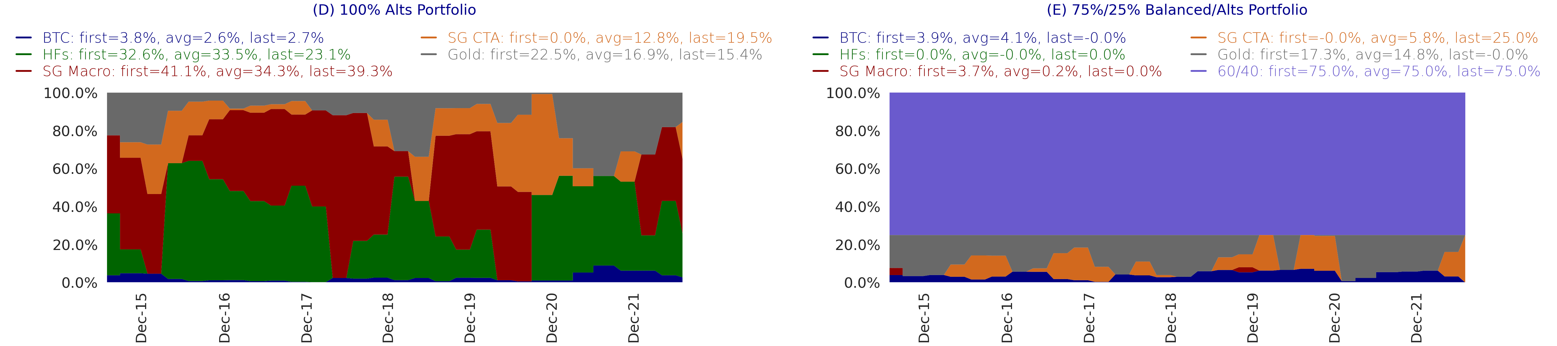
  For each allocation method, I evaluate the following portfolios:
  1. 100% Alts w/o BTC is the portfolio including alternative assets excluding Bitcoin;
  2. 100% Alts with BTC is the portfolio including alternative assets and Bitcoin;
  3. 75%/25% Bal/Alts w/o BTC is the portfolio with fixed allocation to 75% of balanced 60/40 equity/bond portfolio and 25% allocation to alternative assets excluding Bitcoin;
  4. 75%/25% Bal/Alts With BTC is the portfolio with fixed allocation to 75% of balanced 60/40 equity/bond portfolio and 25% allocation to alternative asset classes including Bitcoin.
  Portfolios 1 and 2 enable us to analyze the marginal contribution of including Bitcoin to the investable universe of alternative portfolios. Portfolios 2 and 3 provide with insights into including Bitcoin to alternatives universe for constructing overlays for 60/40 equity/bond portfolio.
  
  Optimal weights
  
  In table below, I show the statistics of time series of optimal weights to Bitcoin produced by the four implemented portfolio optimisers. First, it is notable that all four optimizers produced non-zero weights at all quarterly re-balancing (because the time series minimum is higher than zero) for both portfolios, except for the last quarterly rebalancing of the most diversified 75%/25% portfolio. The optimization of CARA utility produced the highest allocation to Bitcoin for both portfolios, because Bitcoin adds most to the skewness of portfolio returns that is favorable for CARA method. However, the CARA portfolios have the lowest historical allocation to Bitcoin because of declining skewness of its returns. The median of optimisers’ average weights is 2.3% and 4.8% for 100% alts and 75%/25% alts/balanced portfolios, respectively. As a result, including of Bitcoin to the investable universe is beneficial for diversification benefits of broad portfolios.
  
  Figure (4). Minimum, average, maximum, and last weight (as of last quarterly re-balancing on 30 June 2022) to Bitcoin by allocation methods computed using roll-forward simulations from 30 June 2015 to 31 August 2022. Subplot (A) shows the weight in the 100% alternatives portfolio, Subplot (B) shows the weight in the 75%/25% balanced and alts portfolio. ERC is portfolio with equal risk contribution, MaxDiv is portfolio with maximum diversification, MaxSharpe is portfolio with maximum Sharpe ratio, CARA-3 is portfolio with maximum CARA utility under Gaussian mixture model with 3 clusters.
  
  Trailing performance
  
  In below table I show trailing realized Sharpe ratios of simulated optimal portfolios. I add equally weighted portfolio as a benchmark. For 100% alts portfolio w/o and with Bitcoin, the weight of Bitcoin is fixed to 0% and 2%, respectively, while the rest is equally allocated to alternative assets. For 75%/25% balanced/alts portfolio w/o and with Bitcoin, the weight of Bitcoin is fixed to 0% and 0.5%, respectively, the weight of 60/40 portfolio is 75% and rest is equally allocated to alternatives.
  
  First, comparing 100\% alts portfolio w/o and with Bitcoin, we see that adding Bitcoin to the investable universe increased Sharpe ratios over the past periods of 2, 3, 5, 7 years except for the portfolio with maximum Sharpe ratio. The performance over the last year is better for portfolios without Bitcoin. However, I emphasize a robust positive performance of risk-based portfolios with and without Bitcoin in comparison to a poor performance of the benchmark balanced portfolio.
  
  Contrasting 75%/25% balanced/alts portfolio w/o and with Bitcoin, we see that including Bitcoin benefits most of portfolios over all trailing periods. The exceptions include, first, the portfolio with the maximum Sharpe ratio and, second, for the ERC portfolio which slightly under-performs when Bitcoin is added.
  
  A poor relative performance of portfolios with maximum Sharpe ratio highlights the hazard of relying on past data for forecast of future returns. In contrast, out-performers include risk-based methods that rely on the dynamic update of covariance matrices using most recent data.
  
  Figure (5) Sharpe ratios for trailing periods of 1, 2, 3, 5, 7 years starting from 31 August 2021, 2020, 2019, 2017, 2016, respectively, up to 31 August 2022. 60/40 is the benchmark equity/bond balanced portfolio, and EqualWeight w/o and with BTC are equally weighted portfolios with fixed 0% and 2% weights to Bitcoin, respectively.
  
  Conclusion
  
  I present empirical evidence that it has been optimal to include Bitcoin to an investable universe for alternative and blended portfolios, using portfolio diversification metrics. Using roll-forward analysis with dynamic updates of portfolio inputs, I also find that adding Bitcoin have improved performances of optimal portfolios.
  
  I conclude that adding Bitcoin, and more generally, a diversified basket of cryptocurrencies, to the investable universe of broad portfolios may be beneficial for both alternative portfolios and blended balanced/alternative portfolios. I emphasize the need for a robust portfolio allocation method with regular updates of portfolio inputs and re-balancing of portfolio weights.
  
  My favorite allocation method is the optimiser of portfolio diversification metric along with the optimiser of the CARA utility under Gaussian mixture distribution for skewness-seeking investors.
  
  Further details are provided in my paper on SSRN http://ssrn.com/abstract=4217841
  
  Disclaimer
  
  The views and opinions presented in this article and post are mine alone. This research is not an investment advice.
  Share this:
  LinkedIn
  X
  WhatsApp
  Email
  Print
  Posted in Asset Allocation, Crypto, Decentralized Finance, Quantitative Strategies | 2 Comments
- Log-normal Stochastic Volatility Model for Assets with Positive Return-Volatility Correlation – research paper
  
  Posted at 3:04 pm by artursepp, on August 10, 2022
  I am introducing my most recent research on log-normal stochastic volatility model with applications to assets with positive implied volatility skews, such as VIX index, short index ETFs, cryptocurrencies, and some commodities.
  
  Together with Parviz Rakhmonov, we have extended my early work on Karasinski-Sepp log-normal volatility model and we have written an extensive paper with an extra focus on modelling implied volatilities of assets with positive return-volatility correlation in addition to deriving a closed-form solution for option valuation under this model.
  
  Assets with positive implied volatility skews and return-volatility correlations
  
  While it is typical to observe negative correlation between returns of an asset and changes in its implied and realized volatilities, there are in fact many assets with positive return-volatility correlation and, as a consequence, with positive implied volatility skews. In below Figure, I show some representative examples.
  
  (A) The VIX index provides protection against corrections in the S&P 500 index, so that out-of-the-money calls on VIX futures are valuable and demand extra risk-premia than puts.
  
  (B) Short and leveraged short ETFs on equity indices have positive implied volatility skews because of their anti-correlation with underlying equity indices. I use 3x Short Nasdaq ETF with NYSE ticker SQQQ, which is the largest short ETF in US equity market and which has very liquid listed options market.
  
  (C) Cryptocurrencies, including Bitcoin and Ethereum, and “meme” stocks, such as AMC, have positive skews during speculative phases when positive returns feed speculative demand for upside. These self-feeding price dynamics increase the demand for calls following a period of rising prices. However, positive return-volatility correlation tend to reverse once “greed” regime is over and “risk-off” regime prevails.
  
  (D) Gold and commodities in general may have positive volatility skews dependent on supply-demand imbalances, seasonality, etc.
  
  Importantly, the valuation of options on these assets is not feasible using conventional stochastic volatility models applied in practice such as Heston, SABR, Exponential Ornstein-Uhlenbeck stochastic volatility models, because these models fail to be arbitrage-free (forwards and call prices are not martingals). Curiously enough, the topic of no-arbitrage for SV models with positive return-volatility correlation has not received attention in literature, despite a large number of assets with positive return-volatility correlation.
  
  Applications to Options on Cryptocurrencies
  
  Additional, yet important application of our work is the pricing of options on cryptocurrencies, where call and put options with inverse pay-offs are dominant. The advantage of inverse pay-offs for cryptocurrency markets is that all option-related transactions can be handled using units of underlying cryptocurrencies, such as Bitcoin or Ethereum, without using fiat currencies. Critically, since both inverse options (traded on Deribit exchange) and vanilla (traded on CBOE) are traded for cryptocurrencies, a stochastic volatility must satisfy the martingale condition for both money-market-account and inverse measures to exclude arbitrage opportunities between vanilla and inverse options. We show that prices dynamics in our model are martingales under the both inverse and money-market-account measures.
  
  In below Figure, I show the model fit to Bitcoin options observed on 21-Oct-2021 (the period with positive skew) for most liquid maturities of 2 weeks, 1 month, and 2 and 3 months. We see that the model calibrated to Bitcoin options data is able to capture the market implied skew very well across most liquid maturities with only 5 model parameters. The average mean squared error (MSE) is about 1% in implied volatilities, which is mostly within the quoted bid-ask spread. Calibration to ATM region can be further improved using a term structure of the mean volatility or augmenting the SV model with a local volatility part to fit accurately to the implied volatility surface.
  
  Model applications
  
  The quality of model fit is similar for other assets with either positive or negative skews. The main strength of our model is that it can be used for the following purposes.
  1. Cross-sectional no-arbitrage model for different exchanges and options referencing the same underlying.
  2. Model for time series analysis of implied volatility surfaces.
  3. Dynamic valuation model for structured products and option books.
  Further resources
  
  SSRN paper Log-normal Stochastic Volatility Model with Quadratic Drift https://ssrn.com/abstract=2522425
  
  Github project with the example of model implementation in Python: https://github.com/ArturSepp/StochVolModels
  
  Youtube video with lecture I made at Imperial College for model applications for Bitcoin volatility surfaces: https://youtu.be/dv1w_H7NWfQ
  
  Youtube podcast with introduction of the paper and review of Github project with Python analytics for model implementation: https://youtu.be/YHgw0zyzT14
  
  Disclaimer
  
  The views and opinions presented in this article and post are mine alone. This research is not an investment advice.
  Share this:
  LinkedIn
  X
  WhatsApp
  Email
  Print
  Like this:
  Like Loading...
  Posted in Crypto, Python, Volatility Modeling, Volatility Trading | 1 Comment
- Developing systematic smart beta strategies for crypto assets – QuantMinds Presentation
  
  Posted at 3:09 pm by artursepp, on February 23, 2022
  I am delighted to share the video from my QuantMinds presentation that I made in Barcelona in December 2021. Many thanks to QuantMinds organizers for allowing me to share this video. First, it was nice to attend the onsite conference in a while and to meet old friends and colleagues. I was positively surprised by how many people attended. Many thanks to organizers for making it happen during these uncertain times!
  
  I presented a framework for the design of sector-based smart beta indices and products for diversified investing to crypto assets. There are thee challenges to account for when designing a systematic strategy on crypto assets.
  
  First, the data quality is poor indeed. We need to tackle the enormous challenge to accommodate and filter data from multiple data providers. Unlike the traditional asset classes, the market data for public data (such as market cap and traded volumes) can be a source of alpha for systematic strategies.
  
  Second, the time history of data is very short. For example, most of protocol tokens for Decentralized Finance (DeFi) applications were listed during the second half of 2020, which means that we have to ascertain the design and risk-reward profile of a strategy using one year of data.
  
  Third, the liquidity of crypto assets may be insufficient when contrasted with traditional assets. Therefore, we need to carefully design strategies by screening and incorporating the liquidity into the process. One of the challenges is that most crypto exchanges (there are about 30 tier one exchanges) tend to over-estimate their traded volumes.
  
  To overcome these challenges, I constructed a bootstrapping simulation engine which allows to generate joint paths of price and fundamental data for the empirical distributions without breaking the correlation and auto-correlation structure of dependencies in the data.
  Share this:
  LinkedIn
  X
  WhatsApp
  Email
  Print
  Posted in Asset Allocation, Crypto, Decentralized Finance, Quantitative Strategies | 2 Comments
- Paper on Automated Market Making for DeFi: arbitrage-fee exchange between on-chain and traditional markets
  
  Posted at 2:37 pm by artursepp, on September 29, 2021
  I have been delighted to collaborate with Alexander Lipton on a paper where we develop a quantitative approach for making arbitrage-free pricing between decentralized exchanges (DEX), relying on Automated Market Making (AMM), and traditional exchanges, relying on the order book. As a very relevant case for developing central bank digital coins (CBDC) on interoperable blockchains, we simulated our model using high-frequency FX data from a traditional exchange to validate our approach.
  
  This post is a small communication of the background and key results from our paper that can be downloaded from SSRN https://ssrn.com/abstract=3939695
  
  Automated Market Making
  
  Automated market making (AMM) for crypto asset has become one of the most interesting developments in the Decentralized Finance (DeFi) space.
  
  Vitalik Buterin, the founder of Ethereum protocol, originally proposed AMM in 2016 as a concept to exchange on-chain assets on decentralized exchanges which operate entirely on-chain . The purpose was to reduce the spreads and gas fees, that had been excess of 10% at the time. The solution was suggested to create two-sided pools of different coins (for an example, ETH vs BTC) and to fix the exchange rate relative to the pool depth (liquidity).
  
  This concept was formalized by the Uniswap protocol that introduced the so-called constant function market maker (CFMM) using product rule as for marginal pricing of one token vs the other by mean of smart contracts (SC).
  
  The AMM is an interesting concept like a dark pool (in a good sense) where investors can place a large orders and get immediate executions without revealing their intentions prior to their trades.
  
  In Figure 1, I show the relative pricing of a representative USDC-EUDC (US Dollar – Euro) pool (the initial parameters are EUR/USD rate of 1.25) using the three CFMM rules:
  1. Sum rule that allows to swap full balances of one token into another so that the change in the relative rate is a constant.
  2. Product rule that fixes the relative exchange rate inversely proportional to pool balances. Outside of the equilibrium rate of 0.8 EUDC per 1.0 USDC, the relative rate of EUDC will decline or increase faster than the constant exchange rate
  3. Mixed rule with a parameter alpha which is a blended rule between the sum and the product rule.
  Bid/Ask marginal rates
  
  Using the CFMM we can derive the marginal exchange rates as functions of the ratio of the order size to the pool liquidity. This is a very convenient feature that enables to explicitly assign the exchange rate to each order size.
  
  In Figure 2, I show the marginal AMM rates as functions of the CFMM specification. I use the EUR-USD FX spot of 1.25 and equivalent USD-EUR spot of 0.8. Then we can present a representative bid/ask book for trading in both EUDC and USDC from the same USDC-EUDC pool.
  
  It follows that the sum rule enforces no feedback from pool liquidity for the marginal exchange (zero slippage costs) while the product rule produces strong feedback from the pool liquidity (slippage costs proportional to the ratio of traded order to the pool liquidity). By introducing the mixed rule with a parameter alpha between 0 (product rule) and infinity (sum rule), we can design flexible CFMM.
  
  Pool arbitrage
  
  One of the most interesting challenges for on-chain exchanging of different CBDCs is how to avoid arbitrage opportunities between on-chain exchanges and traditional markets. We solve this problem by introducing a pool arbitrageur (either a pool operator or designated market-maker) who follows an optimization problem to arbitrage opportunities between the on-chain pool and traditional markets. Because of the pool arbitrageur, the pool bid/ask spreads for small orders are consistent with a traditional exchange.
  
  We apply our model for simulation of hypothetical CBDC pools using actual high-frequency data FX data. In Figure 3, I show the simulation of USDC-EUDC pool using intraday EUR-USD FX spot rate on 3rd June 2021. For convenience, I normalize the sport FX rate to 1.0 at the start of the trading session. I apply the constant product CFMM.
  
  In the first panel I show the optimal pool balances that are determined by the pool arbitrageur to exclude arbitrage between the pool and the FX spot rate. In the second panel I show the bid/ask spreads for trading 1bp of the pool liquidity. We see that the actual FX spot rate is sandwiched between the AMM bid/ask rates. The final figure is the arbitrage profits.
  
  Application to G-10 currencies
  
  As as a final validation, we also included the volumes for simulations of CBDC pools using the actual FX buy and sell orders. Intraday volumes are normalized so that the pool daily turnover is 100% for each day in our sample of last 3 years of FX data.
  
  In the Figure 4, I show the boxplot of key variables from the simulation of the CBDC pools for G-10 currencies including the Chinese Yuan. I apply the mixed rule CFMM with alpha equal to 5 and the transaction fees of 1bp.
  
  In the first panel, I show the volume-weighted average bid-ask spread. The average spread is about 1.3 across all FX pair, which is competitive to traditional FX markets. The second panel shows the annual P&L (daily P&L multiplied by 260). The last panel shows the Hedged P&L which is produced by hedging the spot exposure or equivalent by allocation to the pool using borrowed CBDCs. It is clear that liquidity providers benefit from both pool fees and the convexity generated by the trading volumes
  
  Summary
  
  Automated market making is one of the core elements for on-chain exchange of digital assets. Of course, one of the most important questions is the arbitrage between on-chain and off-chain exchanges. Alexander Lipton and myself have developed a quantitative approach in this direction.
  
  References
  
  Lipton, A. and Sepp, A., Automated Market-Making for Fiat Currencies (2021). Working Paper, available at SSRN: https://ssrn.com/abstract=3939695
  Share this:
  LinkedIn
  X
  WhatsApp
  Email
  Print
  Like this:
  Like Loading...
  Posted in Crypto, Decentralized Finance, Uncategorized | 2 Comments